Causal Influence Diagram Latex Tutorial
This tutorial will explain how to draw nice-looking causal influence diagrams in LaTeX, using Tikz and the influence-diagrams.sty package.
The file examples.tex produces most of the below diagrams.
Before coding a diagram in Latex, first draw it on paper or in a WYSIWIG editor such as Google slides. Latex is great for professional-looking results, but far from ideal to think in.
Table of contents:
[Advanced] Bent Edges and the Bounding Box
Start with downloading influence-diagrams.sty, and put it in the same folder as your main tex file. In the preamble of your main tex file, include it as
\documentclass{article}
\usepackage[decisionutilitycolor]{influence-diagrams}
\begin{document}
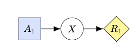
In the main document, add a diagram with the influence-diagram environment:
\begin{influence-diagram}
\node (A) [decision] {$A_1$};
\node (X) [right = of A] {$X$};
\node (U) [right = of X, utility] {$R_1$};
\edge {A} {X};
\edge {X} {U};
\end{influence-diagram}
Nodes are added with the syntax
\node (label) [properties] {text in node};
The label can subsequently be used to position other nodes around the node, and add edges between nodes via \edge {label1} {label2}.
Note that the “properties” field is also used to specify whether a node is a decision or a utility node (by default, it becomes a round chance node).
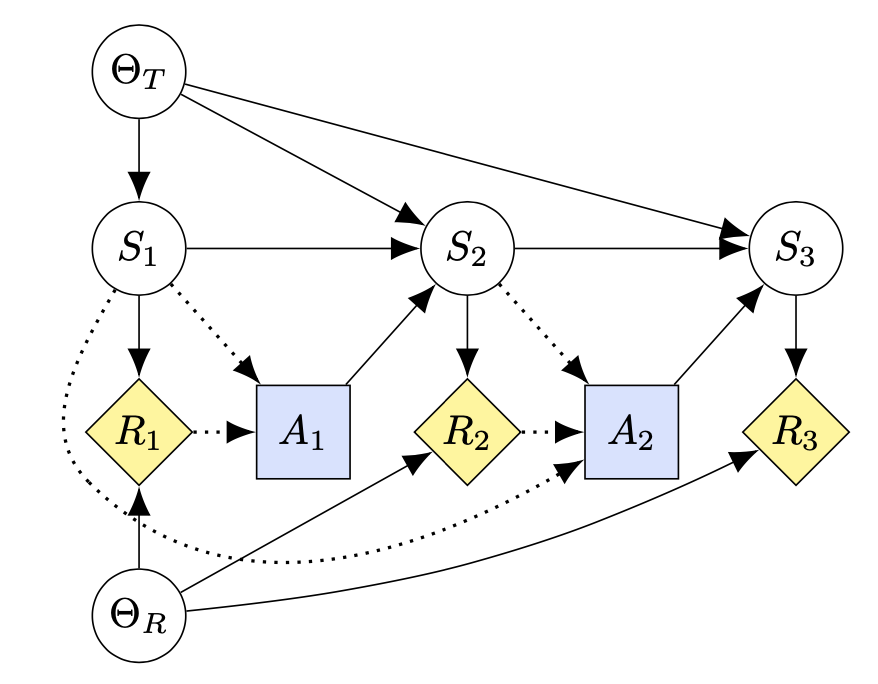
Let’s see how we can make a more complex diagram, with more nodes, dotted information edges, and curved edges to avoid them passing through other nodes.
\begin{influence-diagram}
\node (S1) {$S_1$};
\node (S2) [right = 2 of S1] {$S_2$};
\node (S3) [right = 2 of S2] {$S_3$};
\node (R1) [below = of S1, utility] {$R_1$};
\node (R2) [below = of S2, utility] {$R_2$};
\node (R3) [below = of S3, utility] {$R_3$};
\node (A1) at ($(R1)!0.5!(R2)$) [decision] {$A_1$};
\node (A2) at ($(R2)!0.5!(R3)$) [decision] {$A_2$};
\node (thetaT) [above = of S1] {$\Theta_T$};
\node (thetaR) [below = of R1] {$\Theta_R$};
% Edges (note that multiple labels can be given to each argument)
\edge {S1, thetaR} {R1};
\edge {S2, thetaR} {R2};
\edge {S3} {R3};
\edge {thetaT} {S1};
\edge {thetaT, A1, S1} {S2};
\edge {thetaT, A2, S2} {S3};
% Dotted information edges
\edge[information] {S1, R1} {A1};
\edge[information] {S2, R2} {A2};
% A slightly bent edge, using a different syntax
\path (thetaR) edge[->, bend right=10] (R3);
% A bent information edge, using an invisible helper node
\node (help) [node distance=4mm, below left = of R1, phantom] {};
\draw[information]
(S1) edge[ out=-120, in=135] (help)
(help) edge[->, out=-45, in=-150] (A2);
\end{influence-diagram}
A few things to note:
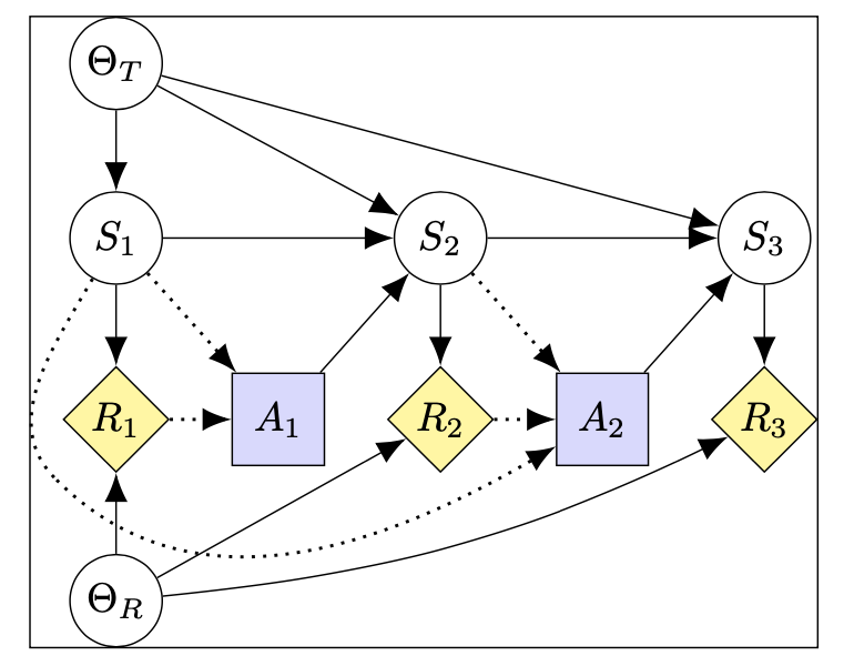
Bent edges can make the bounding box too big because they create invisible control points far from the path and these are included by the bounding box. As a work-around, exclude the path from bounding box calculations by wrapping it in a pgfinterruptboundingbox environment.
To make sure the bounding box includes the bent edge, add one or more extra nodes along the path to be included in the bounding box.
For example, the following code avoids the extra whitespace created by the bent edge in the above diagram:
% This bent edge sticks an invisible control point out too far and messes
% with the bounding box so have the bounding box ignore it
\begin{pgfinterruptboundingbox}
\draw[information]
(S1) edge[in=135, out=-120]
% Bounding box helper
% Place at the bend point or wherever the line is furthest past the
% bounding box.
% Must be manually positioned using pos=(fraction of path length)
% since the bend point is not necessary half way along the path.
node[phantom, pos=0.75] (bbhelper) {}
(help)
(help) edge[->, out=-45, in=-150] (A2);
\end{pgfinterruptboundingbox}
% Place another node at the bbhelper; this time included by the bounding box
% Manually adjust minimum size to compensate for any slight misalignment
% with the bend point of the path and to fully include the path line width.
\node[phantom, minimum size=1pt] at (bbhelper) {};
Add the following just before \end{influence-diagram} to visualize the bounding box:
\draw[black] (current bounding box.south west) rectangle (current bounding box.north east);
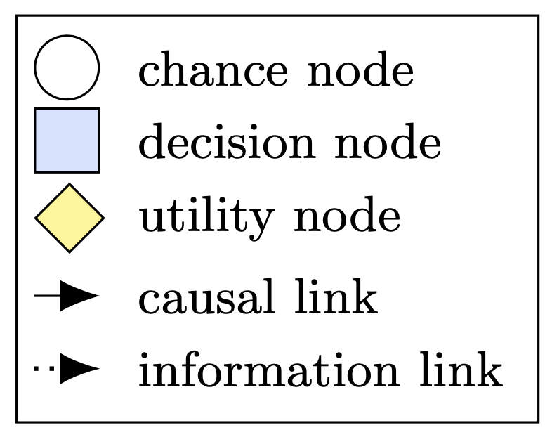
The following code can be used to add a legend to the diagram, explaining the different node types and edges. The command should be used inside influence-diagram environments.
\cidlegend[right = of Y, yshift=-5mm, xshift=1mm]{
\legendrow {} {chance node} \\
\legendrow {decision} {decision node}\\
\legendrow {utility} {utility node}\\
\legendrow[causal] {draw=none} {causal link} \\
\legendrow[information] {draw=none} {information link} }
\edge {causal.west} {causal.east};
\edge[information] {information.west} {information.east};
The legend can be positioned like any other node. For example, this one is positioned right of a node labeled Y, and slightly shifted in both x and y directions.
Each legend row takes a node property as first argument, and a description as a second argument. For the different types of edges, we tell it not to draw the node, and instead give it a label that we can later draw different types of edges around.
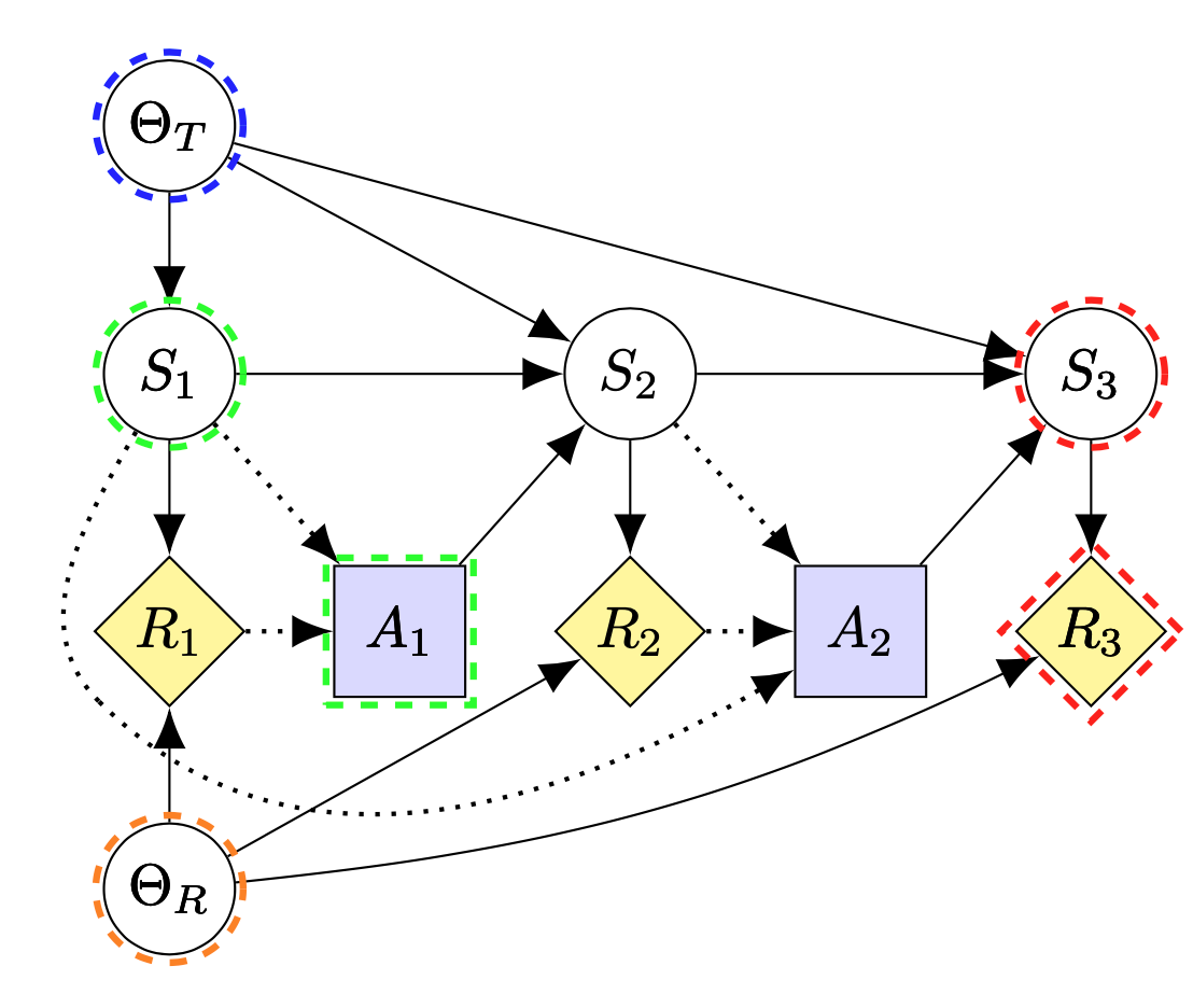
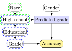
For labeling different types of incentives, there are the commands \fci, \ri, \voi, and \voc. For example, (somewhat non-sensically) adding the following commands to the MDP example above:
\ri{S1}
\ri[rectangle]{A1}
\voi{thetaT}
\fci{S3}
\fci[diamond]{R3}
\voc{thetaR}
produces:
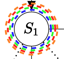
Note that shapes need to be specified manually. If a single node has multiple incentives, the size of the surrounding circles can be adjusted with an optional argument in angle brackets (<1> gives the default size):
\voi<1>{S1}
\ri<2>{S1}
\fci<3>{S1}
\voc<4>{S1}
To annotate decision and utility nodes, supply the correct shape as an optional argument:
\fci[rectangle]{A}
\fci[diamond]<3>{U}
Do not use decision/utility, as these will color the content. The size of the utility annotations typically needs to be manually increased.
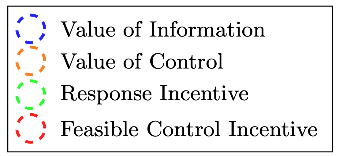
A legend for different types of incentives can be produced with:
\cidlegend{
\legendrow{value of information}{Value of Information}\\
\legendrow{value of control}{Value of Control} \\
\legendrow{response incentive}{Response Incentive}\\
\legendrow{feasible control incentive}{Feasible Control Incentive}}
New types of incentives can be specified by defining new commands on top of the incentive command. For example
\NewDocumentCommand\voci{O{}D<>{1}m}{\incentive{#3}{incentive, gray,#1}{#2}}
defines a new command for gray labels indicating indirect value of control.
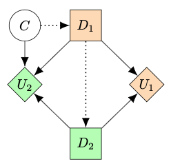
Multi-agent CIDs (MACIDs) can be created with the player1 and player2 keys. Be sure to put these properties after decision or utility, otherwise the color will overwrite.
For additional players, specify their color with e.g. \tikzset{player3/.style = {fill=cyan!30}} in the preamble of the document.
\begin{influence-diagram}
\node (help) [draw=none] {};
\node (P1) [above = of help, decision, player1] {$D_1$};
\node (P2) [below = of help, decision, player2] {$D_2$};
\node (U1) [right = of help, utility, player1] {$U_1$};
\node (U2) [left = of help, utility, player2] {$U_2$};
\node (C) at (U2|-P1) {$C$};
\edge[information] {C} {P1};
\edge[information] {P1} {P2};
\edge {P1,P2} {U1};
\edge {C,P1,P2} {U2};
\end{influence-diagram}
The package currently supports the following options:
For example, importing influence-diagrams.sty with
\usepackage[compact,rectangularnodes] {influence-diagrams}
makes diagrams compact and suitable for text-labels by default.
It is also possible to apply these modifications to a subset of all diagrams. For example
\begin{influence-diagram}
\setcompact
\setrectangularnodes
...
\end{influence-diagram}
will similarly produce a compact diagram with node-shapes suitable for text. The opposite commands are \setnormalsize and \setcircularnodes
The package is based directly on Tikz, so it’s usually possible to google “how to do X in TikZ” to get some good suggestions. Indeed, the influence-diagram environment is just a tikzpicture environment with some default options set.